Global Optimization by Simulating the Motion of a Projectile
Abstract
A new heuristic optimization algorithm is presented based on an analogy with the physical phenomenon of a projectile launched in a conformational space under the influence of a gravitational force. Its implementation simplicity and the option to enhance it with local search methods make it ideal for the optimization of non-linear systems of equations. The algorithm is applied to standard test cases where it successfully recovered known optima and discovered new ones. Suggestion for future development are made since the algorithm proved to be successful enough to warrant further investigation.
Brief Description
Heuristic optimization algorithms have been developed to counter some of the drawbacks of traditional optimization techniques. While a lot of work has been done in the case of local optimization very little progress has been observed in the case of global optimization especially in cases where convexity of the objective function cannot by established. The existence of local optima in objective functions adds to the difficulty of locating a global optimum.
Mathematically, global minimization (optimization) seeks a solution that minimizes a given objective function:
![]()
where ![]() and
and
![]() with
with
![]() and
and
![]() the
lower and upper bounds of each x.
the
lower and upper bounds of each x.
A solution to this type of problems can effectively be handled at low-dimensional problems where rigorous methods based on interval analysis can be applied. The situation changes dramatically as the number of dimensions increases were traditional techniques can only be applied to simple models that can only serve as abstract representation of the systems they represent. In addition solving equations that represent complex phenomena with traditional techniques involves converting these equations (mostly non-linear in form) in form (preferably linear) that can be manipulated by these techniques resulting many times in losses in the accuracy of the achieved solutions. Additional overhead in imposed due to our ignorance of an appropriate starting point (initial value) that could lead to local optima instead of global optima.
In this project an optimization algorithm is presented that was inspired by the physical phenomenon of the motion of a projectile in the conformation space of the objective function under the influence of a gravitational force. The force always attracts objects towards lower potential states that correspond to mimima of the objective function. For all purposes from now on we will be referring to function minimization.
Physical Model of Projectile Flight
It is know from classical mechanics that all objects in nature try and reach an equilibrium state of lowest energy. To illustrate the point if an object of mass m was left to free fall (Figure 1) from a point A at height h in a gravitational field of strength g it will eventually rest (excluding at the moment collision effects with the surface) in the lowest point it can reach - point B. By analogy if the surface represents the objective function and the free falling object is a probe of unitary mass we will expect that the probe eventually will reach the local minimum at B.
This approach will easily be able to locate the local minimum in the area of the initial point A but it needs to be modified in order to avoid being trapped in the minima it reaches so it can increase the chances of exploring other areas of the conformation space of the objective function. One way to avoid being trapped in local minima is to assume elastic collisions with the objective function surface and a big enough initial height to provide the required energy to overcome the maxima around the initial point A.
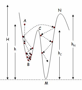
Figure 1. Two dimensional case of an object s free fall in a gravitational field
In the physical world situation the total energy of the mass m is the always the sum of its kinetic and dynamic energy. Assuming elastic collisions with the surface (no loss of energy during collision) the total energy will always remain the same. With figure 1 in mind the total energy ET at point A is only dynamic energy ET =ED=mgh while at point B the object has both dynamic and kinetic
![]()
where v is the velocity of the object at point B. At the lowest point M (global minimum) the object will have only kinetic energy.
The assumption that the collision of the object with the surface is elastic eliminates any energy losses and ensures the object has enough energy to bounce around the conformational space for ever or in our case until and desired minimum (global minimum) is reached. The only requirement is that the initial height h of the object should be higher that the maximum point C of the objective function in the area of the initial point we are interested in locating the global minimum D. Obviously if we were to search larger spaces we need to ensure that the initial height H will be higher than the highest surface point N.
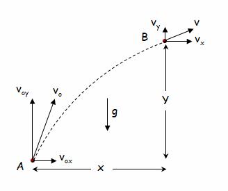
Figure 2. Vector analysis of motion variables in two dimensions
To develop the formulas that will model the phenomenon we need to work out the equations of motion and the collision equations. For the two dimensional case (Figure 2) the equations of motion that show the displacement and velocity of the object after time t for the horizontal axis x x and the normal axis y y have as follows:
![]()
![]()
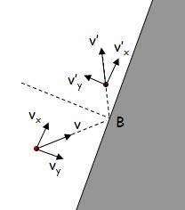
Figure 3. Vector analysis of velocity before and after collision
By applying the theorem of conservation of momentum for the collision at a point B (Figure 3) for an x x axis parallel to the collision surface and a y y axis we have:
A necessary step that also posses the major computational challenge for the method is the calculation of the collision angle that in essence requires the calculation of the derivative of the objective function at the collision point. While the above equations describe the two-dimensional case they can easily be expanded to describe the phenomenon in higher dimensions. A pictorial depiction of a hypothetical trajectory in three dimensions is shown in Figure 4.
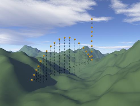
Figure 4. Object trajectory in 3D space
Computational Model of Projectile Flight
Developing the computational algorithm that implements the physical model is a straightforward operation. The steps of the algorithm can be briefed as follows:
Step 1. Random selection of initial point within the boundaries of the conformational space
Step 2. Identify collision point on the objective function surface.
Apply elastic collision rulesStep 3. Repeat the following until a collision occurs:
Calculate the position after time t (increment by a standard time interval Δt)Step 4. Go to step 2 and repeat until the maximum number of execution time is reached
Step 5. Report global minimum
Different positions of the object in a three dimensional example can be seen in Figure 4.
Variations of Computational Model
Given the simplicity of the method variations can be easily developed. Some of them will be described now. A very important assumption in the previous physical and computational representation was that the collision of the moving object with the objective function surface was an elastic collision with no loss of energy. In the physical world though, that is rarely the case. Surfaces and objects are not ideal so we always observe losses of energy. Figure 5 depicts such a situation. While this process might be ideal for local optimization since it will accelerate the time it takes for the object to reach its local minimum energy state (the case will be treated in a follow up publication) it is unlikely to help in reaching the global minimum.
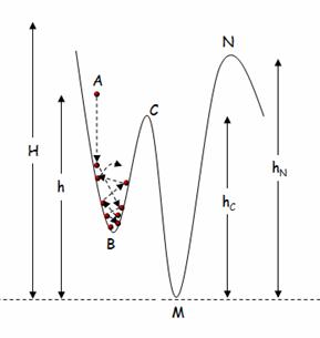
Figure 5. Object trajectory with friction between object and surface
Another observation from the physical world might serve as a more appropriate inspiration for the case of global minimization. As anyone that would observe a free fall of an object knows is usually followed by a breakdown of the object during collision. This can be easily transferred computationally by simulating the object explosion during impact with the objective function surface. Figure 6 depicts such a situation where the object breaks in 5 fragments. One of the fragments follows the trajectory that the original object would follow while the other four scatter in random directions. This way we preserve the initial physical model while at the same time we explore the area in the vicinity of the explosion with the smaller fragments. This operation can be successfully implemented in cases when parallel execution on different CPUs is allowed.
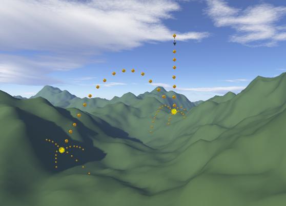
Figure 6. Fragment creation at impact point
A Combined Optimization Approach to Projectile Flight Simulation
Many times in optimization problems we can combine various methods in a complimentary fashion. For instance a global optimization method can organize the selection of random points in the conformational space while a local optimization method locates the local minimum near each point. This way an exploration of the whole space is ensured by the global method while the more reliable local method handles the local features of the space. The projectile flight simulation heuristic can easily be combined with local optimization methods. In Figure 7 a situation is depicted where the projectile method acts as an iterative master process that selects points (collision points) in the conformation space of the objective function. A lower-level method that in this case is a simple gradient descent method takes over at those points and locates the nearest minimum. This way the high-level projectile method ensures the probe object can escape local maxima end eventually retrieve more local minima in the hope of retrieving the global minimum. In essence the global method allows worsening moves (similar to biases introduced by other heuristic methods) that could lead to better global minima.
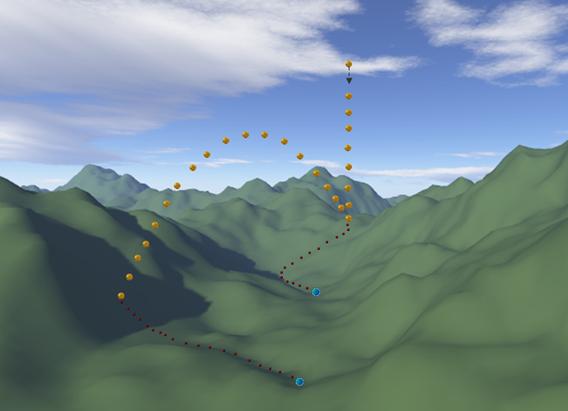
Figure 7. Applying gradient descent methods at impact points
Test Cases
To illustrate the effectiveness of the proposed method the following set of standard problems were selected. Since at the present time the effectiveness of the method in retrieving minima was important its efficiency with respect to time was not considered as all tests were allowed a 24 hour period to execute. All the variations described in the previous section were implemented and tested.
Test Problem 1: Himmelblau function (Reklaitis and Ragsdell, 1983)
All of the nine known solutions [Floudas, and Pardalos, 1999] were retrieved while an additional new one (3.3852 ,0.0739) was observed.
Test Problem 2: Equilibrium Combustion (Meintjes and Morgan, 1990)
The only known solution [Floudas, and Pardalos, 1999] was not retrieved by the method but a new one (0.0009264 0.0812761 0.0510900 0.9990687 0.0001341) was observed and three other could easily be considered valid candidates.
Test Problem 3: (Bullard and Biegler, 1991)
The only known solution [Floudas, and Pardalos, 1999] was retrieved and an additional new one (0.00001,11.47691) was observed.
Test Problem 4: (Ferraris and Tronconi, 1986)
Both know solutions [Floudas, and Pardalos, 1999] were retrieved.
Test Problem 5: (Kearfott and Novoa, 1990)
![]()
One of the two known solutions [Floudas, and Pardalos, 1999] was retrieved while three new ones (0.954,0.954,0.978,0.960,1.189), (0.952,0.922,0.912,0.923,1.362) and (0.936,0.949,0.937,0.969,1.259) were observed.
Conclusions
A probe object is released in the conformational space of the objective function and its motion eventually leads to the discovery of local and global minima. Many alternatives can be implemented based on the availability of computational resources and the problem at hand. As seen in the previous paragraphs the algorithm is easy to describe and implement, whether on a single machine, or in a parallel architecture where execution threads can be assigned to difference processors. Since convergence does not imply efficiency, the practical efficiency of the algorithm was tested by computational experiments. The observed results indicate that the method greatly contributes in the discovery of solutions to non-linear systems of equations. A necessary condition for the application of the method is the existence and computability of the derivatives of the objective function. In addition familiarity with the conformational space will be advantageous if we are to efficiently apply the algorithm. Sharp valleys and mountain tops will require greater initial heights than smoother surfaces (objective functions).
Unfortunate situations where the object can be trapped in repeating the same trajectory can happen when the collision (critical point) angle between the velocity of the object and the tangent to the surface is 90 degrees. In such cases the object will reverse its velocity and follow its up to the collision point trajectory in reverse entering an infinite loop of back and forth between its original free fall point and the critical collision point.
Future work will focus on the modification of the algorithm to successfully adapt the search to the problem s landscape as it executes and improve its effectiveness on a wide category of problems. This way the algorithm will not anymore be blind, in the sense that it will use its current status to modify its search behavior. The modification will be done according to stagnation or progress encountered during search. A new initial height will be established based on the previous information. Additional experimentations that increase the randomness of the method will be explored like for example the introduction of wind that will drift the object in random directions.
Publication
Harkiolakis, N., Global Optimization of Non-Linear Systems of Equations by Simulating the Flight of a Projectile in the Conformational Space , 10th WSEAS International Conference on Mathematical Methods, Computational Techniques and Intelligent Systems, Corfu, Greece, October 26-28, 2008.
Launch the application